Chapter 5 High-Dimensional Data
So far, we have only looked at data structured in a flat/table-like representation (e.g. CSV files). In applied econometrics/statistics, it is common to only work with data sets stored in such format. Data manipulation, filtering, aggregation, etc. presupposes data in a table-like format. Hence, storing data in this format makes perfect sense.
As we observed in the previous chapter, the CSV structure has some disadvantages when representing more complex data in a text file. This is in particular true if the data contains nested observations (i.e., hierarchical structures). While a representation in a CSV file is theoretically possible, it is often far from practical to use other formats for such data. On the one hand, it is likely less intuitive to read the data correctly. On the other hand, storing the data in a CSV file might introduce a lot of redundancy. That is, the identical values of some variables would have to be repeated in the same column. The following code block illustrates this point for a data set on two families ((Murrell 2009), p. 116).
father mother  name     age  gender
               John      33  male
               Julia     32  female
John   Julia   Jack       6  male
John   Julia   Jill       4  female
John   Julia   John jnr   2  male
               David     45  male
               Debbie    42  female
David  Debbie  Donald    16  male
David  Debbie  Dianne    12  female
From simply looking at the data, we can make the best guess which observations belong together (are one family). However, the implied hierarchy is not apparent at first sight. While it might not matter too much that several values have to be repeated several times in this format, given that this data set is so small, the repeated values can become a problem when the data set is much larger. For each time John is repeated in the fathercolumn, we use 4 bytes of memory. Suppose millions of people are in this data set, and we have to transfer this data set very often over a computer network. In that case, these repetitions can become quite costly (as we would need more storage capacity and network resources).
Issues with complex/hierarchical data (with several observation types), intuitive human readability (self-describing), and efficiency in storage, as well as transfer, are all of great importance on the Web. In the context of web technologies, several data formats have been put forward to address these issues. Here, we discuss the two most prominent of these formats: Extensible Markup Language (XML) and JavaScript Object Notation (JSON).
5.1 Deciphering XML
Before going into more technical details, let’s try to figure out the basic logic behind the XML format by simply looking at some raw example data. For this, we turn to the Point Nemo case study in (Murrell 2009). The following code block shows the upper part of the data set downloaded from NASA’s LAS server (here in a CSV-type format).
             VARIABLE : Monthly Surface Clear-sky Temperature (ISCCP) (Celsius)
             FILENAME : ISCCPMonthly_avg.nc
             FILEPATH : /usr/local/fer_data/data/
             BAD FLAG : -1.E+34
             SUBSET   : 48 points (TIME)
             LONGITUDE: 123.8W(-123.8)
             LATITUDE : 48.8S
             123.8W
16-JAN-1994 00    9.200012
16-FEB-1994 00    10.70001
16-MAR-1994 00    7.5
16-APR-1994 00    8.100006
Below, the same data is now displayed in XML format. Note that in both cases, the data is simply stored in a text file. However, it is stored in a format that imposes a different structure on the data.
<?xml version="1.0"?>
<temperatures>
<variable>Monthly Surface Clear-sky Temperature (ISCCP) (Celsius)</variable>
<filename>ISCCPMonthly_avg.nc</filename>
<filepath>/usr/local/fer_data/data/</filepath>
<badflag>-1.E+34</badflag>

<subset>48 points (TIME)</subset>
<longitude>123.8W(-123.8)</longitude>
<latitude>48.8S</latitude>
<case date="16-JAN-1994" temperature="9.200012" />
<case date="16-FEB-1994" temperature="10.70001" />
<case date="16-MAR-1994" temperature="7.5" />
<case date="16-APR-1994" temperature="8.100006" />

...
</temperatures>
What features does the format have? What is its logic? Is there room for improvement? The XML data structure becomes more apparent by using indentation and code highlighting.
<?xml version="1.0"?>
  <temperatures>
    <variable>Monthly Surface Clear-sky Temperature (ISCCP) (Celsius)</variable>
    <filename>ISCCPMonthly_avg.nc</filename>
    <filepath>/usr/local/fer_data/data/</filepath>
    <badflag>-1.E+34</badflag>
    <subset>48 points (TIME)</subset>
    <longitude>123.8W(-123.8)</longitude>
    <latitude>48.8S</latitude>
    <case date="16-JAN-1994" temperature="9.200012" />
    <case date="16-FEB-1994" temperature="10.70001" />
    <case date="16-MAR-1994" temperature="7.5" />
    <case date="16-APR-1994" temperature="8.100006" />

...
  </temperatures>
First, note how special characters are used to define the document’s structure. We notice that < and >, containing some text labels seem to play a key role in defining the structure. These building blocks are called ‘XML tags’. We are free to choose what tags we want to use. In essence, we can define them ourselves to most properly describe the data. Moreover, the example data reveals the flexibility of XML to depict hierarchical structures.
The actual content we know from the CSV-type example above is nested between the ‘temperatures’-tags, indicating what the data is about.
  <temperatures>
...
  </temperatures>
Comparing the actual content between these tags with the CSV-type format above, we further recognize that there are two principal ways to link variable names to values.
    <variable>Monthly Surface Clear-sky Temperature (ISCCP) (Celsius)</variable>
    <filename>ISCCPMonthly_avg.nc</filename>
    <filepath>/usr/local/fer_data/data/</filepath>
    <badflag>-1.E+34</badflag>
    <subset>48 points (TIME)</subset>
    <longitude>123.8W(-123.8)</longitude>
    <latitude>48.8S</latitude>
    <case date="16-JAN-1994" temperature="9.200012" />
    <case date="16-FEB-1994" temperature="10.70001" />
    <case date="16-MAR-1994" temperature="7.5" />
    <case date="16-APR-1994" temperature="8.100006" />
One way is to define opening and closing XML-tags with the variable name and surround the value with them, such as in <filename>ISCCPMonthly_avg.nc</filename>. Another way would be to encapsulate the values within one tag by defining tag attributes such as in <case date="16-JAN-1994" temperature="9.200012" />. In many situations, both approaches can make sense. For example, the way the temperature measurements are encoded in the example data set is based on the tag-attributes approach:
    <case date="16-JAN-1994" temperature="9.200012" />
    <case date="16-FEB-1994" temperature="10.70001" />
    <case date="16-MAR-1994" temperature="7.5" />
    <case date="16-APR-1994" temperature="8.100006" />
We could rewrite this by only using XML tags and no attributes:
  <cases>
    <case>
      <date>16-JAN-1994<date/>
      <temperature>9.200012<temperature/>
    <case/>
    <case>
      <date>16-FEB-1994<date/>
      <temperature>10.70001<temperature/>
    <case/>
    <case>
      <date>16-MAR-1994<date/>
      <temperature>7.5<temperature/>
    <case/>
    <case>
      <date>16-APR-1994<date/>
      <temperature>8.100006<temperature/>
    <case/>
  <cases/>
As long as we follow the basic XML syntax, both versions are valid, and XML parsers can read them equally well.
Note the key differences between storing data in XML format in contrast to a flat, table-like format such as CSV:
- Storing the actual data and metadata in the same file is straightforward (as the above example illustrates). Storing metadata in the first lines of a CSV file (such as in the example above) is theoretically possible. However, by doing so, we break the CSV syntax, and a CSV-parser would likely break down when reading such a file (recall the simple CSV parsing algorithm). More generally, we can represent much more complex (multi-dimensional) data in XML files than what is possible in CSVs. In fact, the nesting structure can be arbitrarily complex as long as the XML syntax is valid.
- The XML syntax is largely self-explanatory and thus both machine-readable and human-readable. That is, not only can parsers/computers more easily handle complex data structures, but human readers can intuitively understand what the data is all about by looking at the raw XML file.
A potential drawback of storing data in XML format is that variable names (in tags) are repeated. Since each tag consists of a couple of bytes, this can be highly inefficient compared to a table-like format where variable names are only defined once. Typically, this means that if the data at hand is only two-dimensional (observations/variables), a CSV format makes more sense.
5.2 Deciphering JSON
In many web applications, JSON serves the same purpose as XML13. An obvious difference between the two conventions is that JSON does not use tags but attribute-value pairs to annotate data. The following code example shows how the same data can be represented in XML or in JSON (example code taken from https://en.wikipedia.org/wiki/JSON):
XML:
<person>
  <firstName>John</firstName>
  <lastName>Smith</lastName>
  <age>25</age>
  <address>
    <streetAddress>21 2nd Street</streetAddress>
    <city>New York</city>
    <state>NY</state>
    <postalCode>10021</postalCode>
  </address>
  <phoneNumber>
    <type>home</type>
    <number>212 555-1234</number>
  </phoneNumber>
  <phoneNumber>
    <type>fax</type>
    <number>646 555-4567</number>
  </phoneNumber>
  <gender>
    <type>male</type>
  </gender>
</person>
JSON:
{"firstName": "John",
  "lastName": "Smith",
  "age": 25,
  "address": {
    "streetAddress": "21 2nd Street",
    "city": "New York",
    "state": "NY",
    "postalCode": "10021"
  },
  "phoneNumber": [
    {
      "type": "home",
      "number": "212 555-1234"
    },
    {
      "type": "fax",
      "number": "646 555-4567"
    }
  ],
  "gender": {
    "type": "male"
  }
}
Note that despite the syntax differences, the similarities regarding the nesting structure are visible in both formats. For example, postalCode is embedded in address, firstname and lastname are at the same nesting level, etc. The following figure, illustrating the nesting structure further illustrates this point. The basic logic of what element belongs to which higher-level element displayed in the tree diagramm is encoded in both the JSON and the XML excerpts shown above.

Figure 5.1: XML tree diagram.
Both XML and JSON are predominantly used to store rather complex, multi-dimensional data. Because they are both human- and machine-readable, these formats are often used to transfer data between applications and users on the Web. Therefore, we encounter these data formats particularly often when we collect data from online sources. Moreover, in the economics/social science context, large and complex data sets (‘Big Data’) often come along in these formats exactly because of the increasing importance of the Internet as a data source for empirical research in these disciplines.
5.3 Parsing XML and JSON in R
As in the case of CSV-like formats, there are several parsers in R that we can use to read XML and JSON data. The following examples are based on the example code shown above (the two text-files persons.json and persons.xml)
# load packages
library(xml2)

# parse XML, represent XML document as R object
xml_doc <- read_xml("persons.xml")
xml_doc
## {xml_document}
## <person>
## [1] <firstName>John</firstName>
## [2] <lastName>Smith</lastName>
## [3] <age>25</age>
## [4] <address>\n <streetAddress>21 2nd Street</streetAddress>\ ...
## [5] <phoneNumber>\n <type>home</type>\n <number>212 555-1234 ...
## [6] <phoneNumber>\n <type>fax</type>\n <number>646 555-4567< ...
## [7] <gender>\n <type>male</type>\n</gender># load packages
library(jsonlite)
# parse the JSON-document shown in the example above
json_doc <- from JSON("persons.json")
# check the structure
str(json_doc)## List of 6
## $ firstName : chr "John"
## $ lastName : chr "Smith"
## $ age : int 25
## $ address :List of 4
## ..$ streetAddress: chr "21 2nd Street"
## ..$ city : chr "New York"
## ..$ state : chr "NY"
## ..$ postalCode : chr "10021"
## $ phoneNumber:'data.frame': 2 obs. of 2 variables:
## ..$ type : chr [1:2] "home" "fax"
## ..$ number: chr [1:2] "212 555-1234" "646 555-4567"
## $ gender :List of 1
## ..$ type: chr "male"5.4 HTML
Recall the data processing example in which we investigated how a webpage can be downloaded, processed, and stored via the R command line. The code constituting a webpage is written in HyperText Markup Language (HTML), designed to be read in a web browser. Thus, HTML is predominantly designed for visual display in browsers, not for storing data. HTML is used to annotate content and define the hierarchy of content in a document to tell the browser how to display (‘render’) this document on the computer screen. Interestingly for us, its structure is very close to that of XML. However, the tags that can be used are strictly pre-defined and are aimed at explaining the structure of a website.
While not intended as a format to store and transfer data, HTMLdocuments (webpages) have de facto become a very important data source for many data science applications both in industry and academia.14 Note how the two key concepts of computer code and digital data (both residing in a text file) are combined in an HTML document. From a web designer’s perspective, HTML is a tool to design the layout of a webpage (and the resulting HTML document is rather seen as code). On the other hand, from a data scientist’s perspective, HTML gives the data contained in a webpage (the actual content) a certain degree of structure which can be exploited to systematically extract the data from the webpage. In the context of HTML documents/webpages as data sources, we thus also speak of ‘semi-structured data’: a webpage can contain an HTML table (structured data) but likely also contains just raw text (unstructured data). In the following, we explore the basic syntax of HTML by building a simple webpage.
5.4.1 Write a simple webpage with HTML
We start by opening a new text-file in RStudio (File->New File->TextFile). On the first line, we tell the browser what kind of document this is with the <!DOCTYPE> declaration set to HTML. In addition, the content of the whole HTML document must be put within <html> and </html>, which represents the ‘root’ of the HTML document. In this, you already recognize the typical (XML-like) annotation style in HTML with so-called HTML tags, starting with < and ending with > or /> in the case of the closing tag, respectively. What is defined between two tags is either another HTML tag or the actual content. An HTML document usually consists of two main components: the head (everything between <head> and </head> ) and the body. The head typically contains metadata describing the whole document like, the title of the document: <title>hello, world</title>. The body (everything between <body> and </body>) contains all kinds of specific content: text, images, tables, links, etc. In our very simple example, we add a few words of plain text. We can now save this text document as mysite.html and open it in a web browser.
     <!DOCTYPE html>

     <html>
         <head>
             <title>hello, world</title>
         </head>
         <body>
             <h2> hello, world </h2>
         </body>
     </html>
From this example, we can learn a few important characteristics of HTML:
- It becomes apparent how HTML is used to annotate/‘mark up’ data/text (with tags) to define the document’s content, structure, and hierarchy. Thus if we want to know what the title of this document is, we have to look for the
<title>-tag. - This systematic structuring adheres to the nesting principle: ‘head’ and ‘body’ are nested within the ‘HTML’ document, at the same hierarchy level. The ‘title’ is defined within the ‘head’, one level lower. In other words, the ‘title’ is a component of the ‘head,’ which is a component of the ‘html’ document. This logic of encapsulating one part in another holds true in all correctly defined HTML documents. This is the type of ‘data structure’ mentioned above, which can be used to extract specific parts of data from HTML documents in a systematic manner.
- We recognize that HTML code essentially expresses what is what in a document (note the similarity of the concept to storing data in XML). HTML code does not contain explicit instructions like programming languages, telling the computer what to do. If an HTML document contains a link to another website, all that is needed, is to define (with HTML tag
<a href=...>) that this is a link. We do not have to explicitly express something like “if the user clicks on a link, then execute this and that…”.
What to do with the HTML document is thus in the hands of the person who works with it. From the data scientist’s perspective, we need to know how to traverse and exploit the structure of an HTML document in order to systematically extract the specific content/data that we are interested in. We thus have to learn how to tell the computer (with R) to extract a specific part of an HTML document. And to do so, we have to acquire a basic understanding of the nesting structure implied by HTML (essentially the same logic as with XML).
One way to think about an HTML document is to imagine it as a tree-diagram, with <html>..</html> as the ‘root’, <head>...</head> and <body>...</body> as the ‘children’ of <html>..</html> (and ‘siblings’ of each other), <title>...</title> as the child of <head>...</head>, etc. Figure 5.2 illustrates this point.
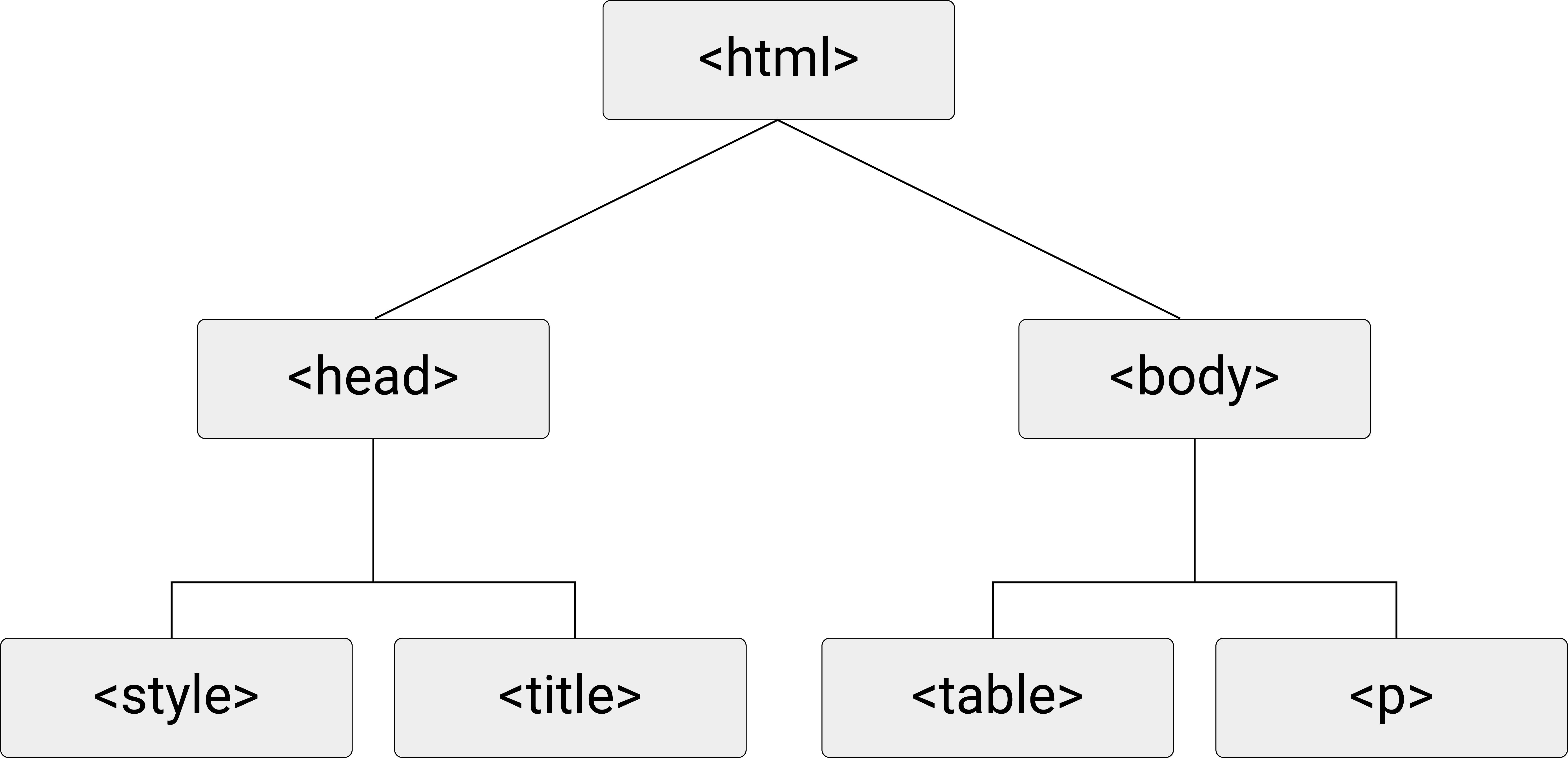
Figure 5.2: HTML (DOM) tree diagram.
The illustration of the nested structure can help to understand how we can instruct the computer to find/extract a specific part of the data from such a document. In the following exercise, we revisit the example shown in the chapter on data processing to do exactly this.
5.4.2 Two ways to read a webpage into R
In this example, we look at Wikipedia’s Economy of Switzerland page, which contains the table depicted in Figure 5.3.
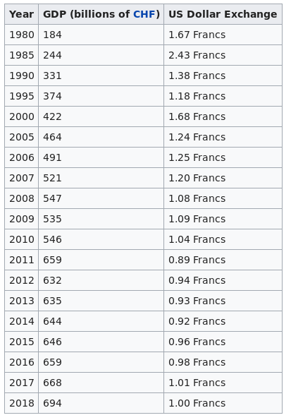
Figure 5.3: Source: https://en.wikipedia.org/wiki/Economy_of_Switzerland.
As in the example shown in the data processing chapter (‘world population clock’), we first tell R to read the lines of text from the HTML document that constitutes the webpage.
swiss_econ <- readLines("https://en.wikipedia.org/wiki/Economy_of_Switzerland")## Warning in
## readLines("https://en.wikipedia.org/wiki/Economy_of_Switzerland"):
## incomplete final line found on
## 'https://en.wikipedia.org/wiki/Economy_of_Switzerland'And we can check if everything worked out well by having a look at the first lines of the web page’s HTML code:
head(swiss_econ)## [1] "<!DOCTYPE html>"
## [2] "<html class=\"client-nojs\" lang=\"en\" dir=\"ltr\">"
## [3] "<head>"
## [4] "<meta charset=\"UTF-8\"/>"
## [5] "<title>Economy of Switzerland - Wikipedia</title>"
## [6] "<script>document.documentElement.className=\"client-js\";RLCONF={\"wgBreakFrames\":false,\"wgSeparatorTransformTable\":[\"\",\"\"],\"wgDigitTransformTable\":[\"\",\"\"],\"wgDefaultDateFormat\":\"dmy\",\"wgMonthNames\":[\"\",\"January\",\"February\",\"March\",\"April\",\"May\",\"June\",\"July\",\"August\",\"September\",\"October\",\"November\",\"December\"],\"wgRequestId\":\"5196e138-1f0f-4e32-98c5-559644dcf716\",\"wgCSPNonce\":false,\"wgCanonicalNamespace\":\"\",\"wgCanonicalSpecialPageName\":false,\"wgNamespaceNumber\":0,\"wgPageName\":\"Economy_of_Switzerland\",\"wgTitle\":\"Economy of Switzerland\",\"wgCurRevisionId\":1125705546,\"wgRevisionId\":1125705546,\"wgArticleId\":27465,\"wgIsArticle\":true,\"wgIsRedirect\":false,\"wgAction\":\"view\",\"wgUserName\":null,\"wgUserGroups\":[\"*\"],\"wgCategories\":[\"CS1 maint: archived copy as title\",\"CS1 German-language sources (de)\",\"Articles with German-language sources (de)\",\"Webarchive template wayback links\",\"Articles with French-language sources (fr)\",\"Articles with short description\",\"Short description is different from Wikidata\","The next thing we do is to look at how we can filter the webpage for certain information. For example, we search in the source code for the line that contains the part of the webpage with the table showing data on the Swiss GDP:
line_number <- grep('US Dollar Exchange', swiss_econ)Recall: we ask R on which line in swiss_econ (the source code stored in RAM) the text US Dollar Exchange is and store the answer (the line number) in RAM under the variable name line_number.
Then, we check on which line the text was found.
line_number## [1] 233Knowing that the R object swiss_econ is a character vector (with each element containing one line of HTML code as a character string), we can look at this particular code:
swiss_econ[line_number]## [1] "<th>US Dollar Exchange"Note that this rather primitive approach is ok to extract a chunk of code from an HTML document, but it is far from practical when we want to extract specific parts of data (the actual content, not including HTML code). So far, we have completely ignored that the HTML tags give some structure to the data in this document. That is, we simply have read the entire document line by line, not making a difference between code and data. The approach to filter the document could have equally well been taken for a plain text file.
If we want to exploit the structure given by HTML, we need to parse the HTML when reading the webpage into R. We can do this with the help of functions provided in the rvest package:
# install package if not yet installed
# install.packages("rvest")

# load the package
library(rvest)
After loading the package, we read the webpage into R, but this time using a function that parses the HTML code:
# parse the webpage, show the content
swiss_econ_parsed <- read_html("https://en.wikipedia.org/wiki/Economy_of_Switzerland")
swiss_econ_parsed
## {html_document}
## <html class="client-nojs" lang="en" dir="ltr">
## [1] <head>\n<meta http-equiv="Content-Type" content="text/html ...
## [2] <body class="skin-vector-legacy mediawiki ltr sitedir-ltr ...Now we can easily separate the data/text from the HTML code. For example, we can extract the HTML table containing the data we are interested in as data frames.
tab_node <- html_node(swiss_econ_parsed, xpath = "//*[@id='mw-content-text']/div/table[2]")
tab <- html_table(tab_node)
tab
## # A tibble: 19 × 3
## Year `GDP (billions of CHF)` `US Dollar Exchange`
## <int> <int> <chr>
## 1 1980 184 1.67 Francs
## 2 1985 244 2.43 Francs
## 3 1990 331 1.38 Francs
## 4 1995 374 1.18 Francs
## 5 2000 422 1.68 Francs
## 6 2005 464 1.24 Francs
## 7 2006 491 1.25 Francs
## 8 2007 521 1.20 Francs
## 9 2008 547 1.08 Francs
## 10 2009 535 1.09 Francs
## 11 2010 546 1.04 Francs
## 12 2011 659 0.89 Francs
## 13 2012 632 0.94 Francs
## 14 2013 635 0.93 Francs
## 15 2014 644 0.92 Francs
## 16 2015 646 0.96 Francs
## 17 2016 659 0.98 Francs
## 18 2017 668 1.01 Francs
## 19 2018 694 1.00 Francs