Chapter 4 Data Storage and Data Structures
A core part of the practical skills covered in this book has to do with writing, executing, and storing computer code (i.e., instructions to a computer in a language that it understands) as well as storing and reading data. The way data is typically stored on a computer follows quite naturally from the outlined principles of how computers process data (both technically speaking and in terms of practical applications). Based on a given standard of how 0s and 1s are translated into the more meaningful symbols we see on our keyboard, we simply write data (or computer code) to a text file and save this file on the hard-disk drive of our computer. Again, what is stored on disk is in the end only consisting of 0s and 1s. But, given the standards outlined in the previous chapter, these 0s and 1s properly map to characters that we can understand when reading the file again from the disk and looking at its content on our computer screen.
4.1 Unstructured data in text files
In the simplest case, we want to store a text literally. For example, we store the following phrase
Hello, World!
in a text file named helloworld.txt. Technically, this means that we allocate a block of computer memory to helloworld.txt (a ‘file’ is, in the end, a block of computer memory). The ending .txt indicates to the operating system of our computer what kind of data is stored in this file. When clicking on the file’s symbol, the operating system will open the file (read it into RAM) with the default program assigned to open .txt-files (for example, Atom or RStudio). That is, the format of a file says something about how to interpret the 0s and 1s. If the text editor displays Hello World! as the content of this file, the program correctly interprets the 0s and 1s as representing plain text and uses the correct character encoding to convert the raw 0s and 1s yet again to symbols that we can read more easily. Similarly, we can show the content of the file in the command-line terminal (here OSX or Linux):
cat helloworld.txt## Hello World!Or, from the R-console:
system("cat helloworld.txt")However, we can also use a command-line program (here, xxd) to display the content of helloworld.txt without actually ‘translating’ it into ASCII characters.7 That is, we can directly look at how the content looks like as 0s and 1s:
xxd -b helloworld.txt## 00000000: 01001000 01100101 01101100 01101100 01101111 00100000 Hello
## 00000006: 01010111 01101111 01110010 01101100 01100100 00100001 World!Similarly, we can display the content in hexadecimal values:
xxd helloworld.txt## 00000000: 4865 6c6c 6f20 576f 726c 6421 Hello World!Next, consider the text file hastamanana.txt, which was written and stored with another character encoding. When looking at the content, assuming the now common UTF-8 encoding, the content seems a little odd:
cat hastamanana.txt## Hasta Ma?ana!We see that it is a short phrase written in Spanish. Strangely it contains the character ? in the middle of a word. The occurrence of special characters in unusual places of text files is an indication of using the wrong character encoding to display the text. Let’s check what the file’s encoding is.
file -b hastamanana.txt## ISO-8859 textThis tells us that the file is encoded with ISO-8859 (‘Latin1’), a character set for several Latin languages (including Spanish). Knowing this, we can check how the content looks like when we change the encoding to UTF-8 (which then properly displays the content on the screen)8:
iconv -f iso-8859-1 -t utf-8 hastamanana.txt | cat## Hasta Mañana!When working with data, we must therefore ensure that we apply the proper standards to translate the binary coded values into a character/text representation that is easier to understand and work with. In recent years, much more general (or even ‘universal’) standards have been developed and adopted worldwide, particularly UTF-8. Thus, if we deal with recently generated data sets, we usually can expect that they are encoded in UTF-8, independent of the data’s country of origin. However, when working on a research project with slightly older data sets from different sources, encoding issues still occur quite frequently. It is thus crucial to understand the origin of the problem early on when the data seem to display weird characters. Encoding issues are among the most basic problems that can occur when importing data.
So far, we have only looked at very simple examples of data stored in text files, essentially only containing short phrases of text. Nevertheless, the most common formats of storing and transferring data (CSV, XML, JSON, etc.) build on exactly the same principle: characters in a text-file. The difference between such formats and the simple examples above is that their content is structured in a very specific way. That is, on top of the lower-level conversion of 0s and 1s into characters/text, we add another standard, a data format, giving the data more structure, making it even simpler to interpret and work with the data on a computer. Once we understand how data is represented at a low level (the topic of the previous chapter), it is much easier to understand and distinguish different forms of storing structured data.
4.2 Structured data formats
As nicely pointed out by Murrell (2009), the most commonly used software today is designed in a very ‘user-friendly’ way, leading to situations in which we as users are ‘told’ by the computer what to do (rather than the other way around). A prominent symptom of this phenomenon is that specific software is automatically assigned to open files of specific formats, so we don’t have to bother about what the file’s format actually is but only have to click on the icon representing the file.
However, if we actually want to engage seriously with a world driven by data, we have to go beyond the habit of simply clicking on (data-)files and let the computer choose what to do with it. Since most common formats to store data are in essence text files (in research contexts usually in ASCII or UTF-8 encoding), a good way to start engaging with a data set is to look at the raw text file containing the data in order to get an idea of how the data is structured.
For example, let’s have a look at the file ch_gdp.csv. When opening the file in a text editor we see the following:
year,gdp_chfb
1980,184
1985,244
1990,331
1995,374
2000,422
2005,464
At first sight, the file contains a collection of numbers and characters. Having a closer look, certain structural features become apparent. The content is distributed over several rows, with each row containing a comma character (,). Moreover, the first row seems systematically different from the following rows: it is the only row containing alphabetical characters, all the other rows contain numbers. Rather intuitively, we recognize that the specific way in which the data in this file is structured might, in fact, represent a table with two columns: one with the variable year describing the year of each observation (row), the other with the variable gdp_chfb with numerical values describing another characteristic of each observation/row (we can guess that this variable is somehow related to GDP and CHF/Swiss francs).
The question arises, how do we work with this data? Recall that it is simply a text file. All the information stored in it is displayed above. How could we explain to the computer that this is a table with two columns containing two variables describing six observations? We would have to come up with a sequence of instructions/rules (i.e., an algorithm) of how to distinguish columns and rows when all that a computer can do is sequentially read one character after the other (more precisely one 0/1 after the other, representing characters).
This algorithm could be something along the lines of:
- Start with an empty table consisting of one cell (1 row/column).
- While the end of the input file is not yet reached, do the following:
Read characters from the input file, and add them one-by-one to the current cell.
If you encounter the character ‘
,’, ignore it, create a new field, and jump to the new field. If you encounter the end of the line, create a new row and jump to the new row.
Consider the usefulness of this algorithm. It would certainly work quite well for the particular file we are looking at. But what if another file we want to read data from does not contain any ‘,’ but only ‘;’? We would have to tweak the algorithm accordingly. Hence, again, it is extremely useful if we can agree on certain standards of how data structured as a table/matrix is stored in a text file.
4.2.1 CSVs and fixed-width format
Incidentally, the example we are looking at here is in line with such a standard, i.e., Comma-Separated Values (CSV, therefore .csv). In technical terms, the simple algorithm outlined above is a CSV parser. A CSV parser is a software component which takes a text file with CSV standard structure as input and builds a data structure in the form of a table (represented in RAM). If the input file does not follow the agreed-on CSV standard, the parser will likely fail to properly ‘parse’ (read/translate) the input.
CSV files are very often used to transfer and store data in a table-like format. They essentially are based on two rules defining the structure of the data: commas delimit values/fields in a row and the end of a line indicates the end of a row.9
The comma is clearly visible when looking at the raw text content of ch_gdp.csv. However, how does the computer know that a line is ending? By default most programs to work with text files do not show an explicit symbol for line endings but instead display the text on the next line. Under the hood, these line endings are, however, non-printable characters. We can see this when investigating ch_gdp.csv in the command-line terminal (via xxd):
xxd ch_gdp.csv## 00000000: efbb bf79 6561 722c 6764 705f 6368 6662 ...year,gdp_chfb
## 00000010: 0d31 3938 302c 3138 340d 3139 3835 2c32 .1980,184.1985,2
## 00000020: 3434 0d31 3939 302c 3333 310d 3139 3935 44.1990,331.1995
## 00000030: 2c33 3734 0d32 3030 302c 3432 320d 3230 ,374.2000,422.20
## 00000040: 3035 2c34 3634 05,464When comparing the hexadecimal values with the characters they represent on the right side, we recognize that a full stop (.) is printed to the output right before every year. Moreover, when inspecting the hexadecimal code, we recognize that this . corresponds to 0d in the hexadecimal code. 0d is indeed the sequence of 0s and 1 indicating the end of a line. Because this character does not actually correspond to a symbol printed on the screen, it is replaced by . in the printed output of the text.10
While CSV files have become a very common way to store ‘flat’/table-like data in plain text files, several similar formats can be encountered in practice. Most commonly they either use a different delimiter (for example, tabs/white space) to separate fields in a row, or fields are defined to consist of a fixed number of characters (so-called fixed-width formats). In addition, various more complex standards to store and transfer digital data are widely used to store data. Particularly in the context of web data (data stored and transferred online), files storing data in these formats (e.g., XML, JSON, YAML, etc.) are in the end, just plain text files. However, they contain a larger set of special characters/delimiters (or combinations of these) to indicate the structure of the data stored in them.
4.3 Units of information/data storage
The question of how to store digital data on computers also raises the question of storage capacity. Because every type of digital data can, in the end, only be stored as 0s and 1s, it makes perfect sense to define the smallest unit of information in computing as consisting of either a 0 or a 1. We call this basic unit a bit (from binary digit; abbrev. ‘b’). Recall that the decimal number 139 corresponds to the binary number 10001011. To store this number on a hard disk, we require a capacity of 8 bits or one byte (1 byte = 8 bits; abbrev. ‘B’). Historically, one byte encoded a single character of text (i.e., in the ASCII character encoding system). 4 bytes (or 32 bits) are called a word. The following figure illustrates this point.

Figure 4.1: Byte and bit.
Bigger units for storage capacity usually build on bytes:
- \(1 \text{ kilobyte (KB)} = 1000^{1} \approx 2^{10} \text{ bytes}\)
- \(1 \text{ megabyte (MB)} = 1000^{2} \approx 2^{20} \text{ bytes}\)
- \(1 \text{ gigabyte (GB)} = 1000^{3} \approx 2^{30} \text{ bytes}\)
- \(1 \text{ terabyte (TB)} = 1000^{4} \approx 2^{40} \text{ bytes}\)
- \(1 \text{ petabyte (PB)} = 1000^{5} \approx 2^{50} \text{ bytes}\)
- \(1 \text{ exabyte (EB)} = 1000^{6} \approx 2^{60} \text{ bytes}\)
- \(1 \text{ zettabyte (ZB)} = 1000^{7} \approx 2^{70} \text{ bytes}\)
\(1 ZB = 1000000000000000000000\text{ bytes} = 1 \text{ billion terabytes} = 1 \text{ trillion gigabytes}.\)
4.4 Data structures and data types in R
So far, we have focused on how data is stored on the hard disk. That is, we discovered how ’0’s and ’1’s correspond to characters (using specific standards: character encodings), how a sequence of characters in a text file is a useful way to store data on a hard disk, and how specific standards are used to structure the data in a meaningful way (using special characters). When thinking about how to store data on a hard disk, we are usually concerned with how much space (in bytes) the data set needs, how well it is transferable/understandable, and how well we can retrieve information from it. All of these aspects go into the decision of what structure/format to choose etc.
However, none of these considers how we actively work with the data. For example, when we want to sum up the gdp_chfb column in ch_gdp.csv (the table example above), do we actually work within the CSV data structure? The answer is usually no.
Recall from the basics of data processing that data stored on the hard disk is loaded into RAM to work with (analysis, manipulation, cleaning, etc.). The question arises as to how data is structured in RAM? That is, what data structures/formats are used to work with the data actively?
We distinguish two basic characteristics:
- Data types: integers; real numbers (‘numeric values’, floating point numbers); text (‘string’, ‘character values’).
- Basic data structures in RAM:
- Vectors
- Factors
- Arrays/matrices
- Lists
- Data frames (very
R-specific)
Depending on the data structure/format stored in on the hard disk, the data will be more or less usefully represented in one of the above structures in RAM. For example, in the R language it is quite common to represent data stored in CSVs on disk as data frames in RAM. Similarly, it is quite common to represent a more complex format on disk, such as JSON, as a nested list in RAM.
Importing data from the hard disk (or another mass storage device) into RAM in order to work with it in R essentially means reading the sequence of characters (in the end, of course, 0s and 1s) and mapping them, given the structure they are stored in, into one of these structures for representation in RAM.11.
4.4.1 Data types
From the previous chapters, we know that digital data (0s and 1s) can be interpreted in different ways depending on the format it is stored in. Similarly, data loaded into RAM can be interpreted differently by R depending on the data type. Some operators or functions in R only accept data of a specific type as arguments. For example, we can store the numeric values 1.5 and 3 in the variables a and b, respectively.
a <- 1.5
b <- 3
R interprets this data as type double (class ‘numeric’; a ‘double precision floating point number’):
typeof(a)## [1] "double"class(a)## [1] "numeric"Given that these bytes of data are interpreted as numeric, we can use operators (here: math operators) that can work with such types:
a + b## [1] 4.5If we define a and b as follows, R will interpret the values stored in a and b as text (character).
a <- "1.5"
b <- "3"typeof(a)## [1] "character"class(a)## [1] "character"Now the same line of code as above will result in an error:
a + b## Error in a + b: non-numeric argument to binary operatorThe reason is that an operator + expects numeric or integer values as arguments. When importing data sets with many different variables (columns), it is thus necessary to ensure that each column is interpreted in the intended way. That is, we have to make sure R is assigning the right type to each of the imported variables. Usually, this is done automatically. However, with large and complex data sets, the automatic recognition of data types when importing data can fail when the data is not perfectly cleaned/prepared (in practice, this is very often the case).
4.4.2 Data structures
For now, we have only looked at individual bytes of data. An entire data set can consist of gigabytes of data containing text and numeric values. How can such collections of data values be represented in R? Here, we look at the main data structures implemented in R. All of these structures will play a role in some of the hands-on exercises.
4.4.2.1 Vectors
Vectors are collections of values of the same type. They can contain either all numeric values or all character values. We will use the following symbol to refer to vectors.
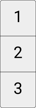
Figure 4.2: Illustration of a numeric vector.
For example, we can initiate a character vector containing the names of persons:
persons <- c("Andy", "Brian", "Claire")
persons
## [1] "Andy" "Brian" "Claire"And we can initiate a numeric vector with the age of these persons:
ages <- c(24, 50, 30)
ages
## [1] 24 50 304.4.2.2 Factors
Factors are sets of categories. Thus, the values come from a fixed set of possible values.
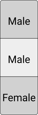
Figure 4.3: Illustration of a factor.
For example, we might want to initiate a factor that indicates the gender of a number of people.
gender <- factor(c("Male", "Male", "Female"))
gender
## [1] Male Male Female
## Levels: Female Male4.4.2.3 Matrices/Arrays
Matrices are two-dimensional collections of values, arrays of higher-dimensional collections of values of the same type. For an illustration, consider the following \(3\times3\) integer matrix and the \(3\times3\times3\) integer array.
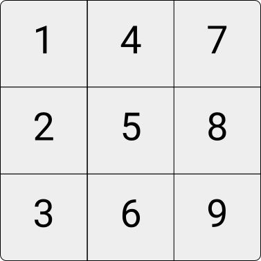
Figure 4.4: Illustration of an integer matrix.
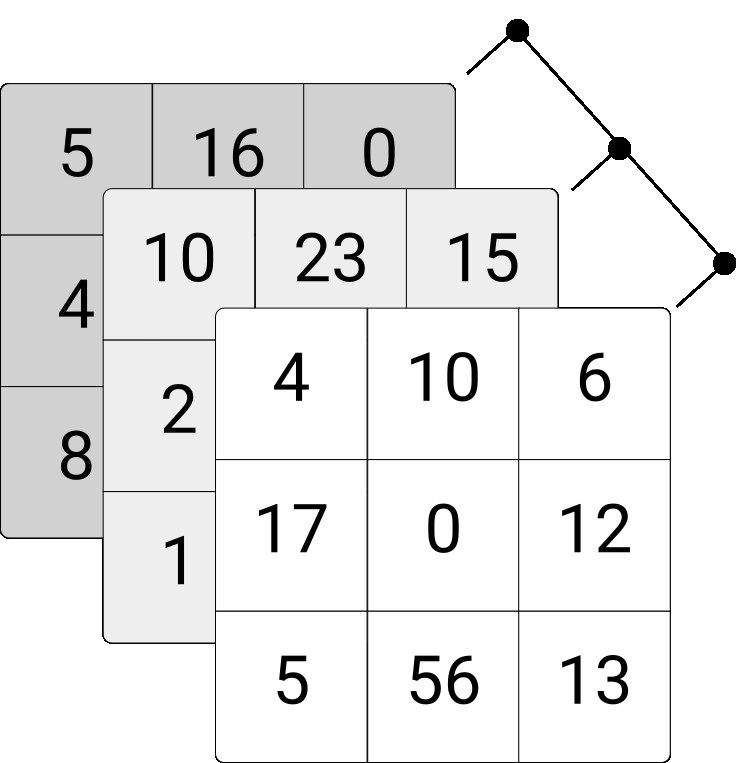
Figure 4.5: Illustration of three-dimensional integer array.
In R, we can, for example, initiate a three-row/three-column integer matrix as follows.
my_matrix <- matrix(1:9, nrow = 3)
my_matrix
## [,1] [,2] [,3]
## [1,] 1 4 7
## [2,] 2 5 8
## [3,] 3 6 9Similarly, we can initiate a three-dimensional array via the array()-function as shown below. Note that instead of defining only the numbers of rows (columns), you need to define the number of elements in each dimension via the dim-parameter.
my_array <- array(1:27, dim = c(3,3,3))
my_array## , , 1
##
##      [,1] [,2] [,3]
## [1,]    1    4    7
## [2,]    2    5    8
## [3,]    3    6    9
##
## , , 2
##
## [,1] [,2] [,3]
## [1,] 10 13 16
## [2,] 11 14 17
## [3,] 12 15 18
##
## , , 3
##
## [,1] [,2] [,3]
## [1,] 19 22 25
## [2,] 20 23 26
## [3,] 21 24 27We can access parts of matrices and arrays via indexing implemented with the []-syntax. For example, select a particular row, column, or individual element of a matrix.
# Select the first row
my_matrix[1,]## [1] 1 4 7# Select the second column
my_matrix[,2]## [1] 4 5 6# Select the value in the second column, third row.
my_matrix[3,2]## [1] 6Following the same syntax, we can access specific parts of an array. Note, though, that we need to consider the correct number of dimensions of the corresponding array object. In the example of above, we have generated three-dimensional array, hence there needs to be three parts within the [].
# Select the first rows
my_array[1,,]## [,1] [,2] [,3]
## [1,] 1 10 19
## [2,] 4 13 22
## [3,] 7 16 25# Select the "third matrix"
my_array[,,3]## [,1] [,2] [,3]
## [1,] 19 22 25
## [2,] 20 23 26
## [3,] 21 24 27# Select the "last" element in the array
my_array[3,3,3]## [1] 274.4.2.4 Data frames, tibbles, and data tables
Data frames are the typical representation of a (table-like) data set in R. Each column can contain a vector of a given data type (or a factor), but all columns need to be of identical length. Thus in the context of data analysis, we would say that each row of a data frame contains an observation, and each column contains a characteristic of this observation.

Figure 4.6: Illustration of a data frame.
The historical implementation of data frames in R is not very appropriate to work with large datasets. 12 These days there are new implementations of the data frame concept in R provided by different packages, which aim at making data processing based on ‘data frames’ faster. One is called tibbles, implemented and used in the tidyverse packages. The other is called data table, implemented in the data. table-package. In this book, we will encounter primarily classical data. frame and tibble (however, there will also be some hints to tutorials with data. table). In any case, once we understand data frames in general, working with tibble and data. table is quite easy because functions that accept classical data frames as arguments also accept those newer implementations.
Here is how we define a data frame in R, based on the examples of vectors and factors shown above.
df <- data.frame(person = persons, age = ages, gender = gender)
df## person age gender
## 1 Andy 24 Male
## 2 Brian 50 Male
## 3 Claire 30 Female4.4.2.5 Lists
Unlike data frames, lists can contain different data types in each element. Moreover, they even can contain different data structures of different dimensions in each element. For example, a list could contain different other lists, data frames, and vectors with differing numbers of elements.
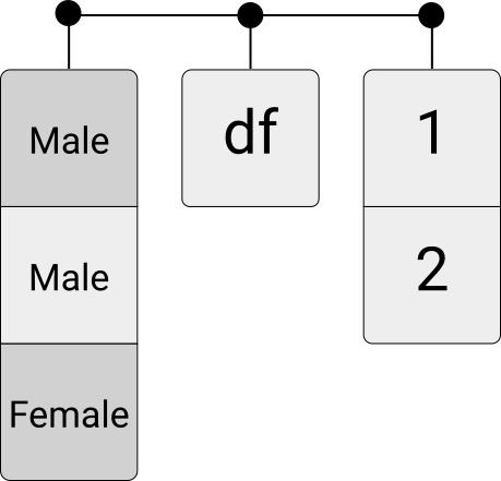
Figure 4.7: Illustration of a list.
This flexibility can easily be demonstrated by combining some of the data structures created in the examples above:
my_list <- list(my_array, my_matrix, df)
my_list## [[1]]
## , , 1
##
##      [,1] [,2] [,3]
## [1,]    1    4    7
## [2,]    2    5    8
## [3,]    3    6    9
##
## , , 2
##
##      [,1] [,2] [,3]
## [1,]   10   13   16
## [2,]   11   14   17
## [3,]   12   15   18
##
## , , 3
##
##      [,1] [,2] [,3]
## [1,]   19   22   25
## [2,]   20   23   26
## [3,]   21   24   27
##
##
## [[2]]
## [,1] [,2] [,3]
## [1,] 1 4 7
## [2,] 2 5 8
## [3,] 3 6 9
##
## [[3]]
##   person age gender
## 1   Andy  24   Male
## 2  Brian  50   Male
## 3 Claire 30 FemaleTo be precise, this program shows both the raw binary content as well as its ASCII representation.↩︎
Note that changing the encoding in this way only works well if we know what the original encoding of the file is (i.e., the encoding used when the file was initially created). While the
filecommand above simply tells us what the original encoding was, it has to make an educated guess in most cases (as the original encoding is often not stored as metadata describing a file). See, for example, the Mozilla Charset Detectors.↩︎In addition, if a field contains itself a comma (the comma is part of the data), the field needs to be surrounded by double-quotes (
"). If a field contains double-quotes it also has to be surrounded by double-quotes, and the double quotes in the field must be preceded by an additional double-quote.↩︎The same applies to other sequences of
0s and1s that do not correspond to a printable character.↩︎In the chapter on data gathering and data import, we will cover this crucial step in detail.↩︎
In the early days of R, this was not an issue because datasets that are rather large by today’s standards (in the Gigabytes) could not have been handled properly by normal computers anyway (due to a lack of RAM).↩︎