Chapter 9 Data Preparation

Importing a dataset properly is just the first of several milestones until an analysis-ready dataset is generated. In some cases, cleaning the raw data is a necessary step to facilitate/enable proper parsing of the data set to import it. However, most of the cleaning/preparation (‘wrangling’) with the data follows after properly parsing structured data. Many aspects of data wrangling are specific to certain datasets and an entire curriculum could be filled with different approaches and tools to address specific problems. Moreover, proficiency in data wrangling is generally a matter of experience in working with data, gained over many years. Here, we focus on two quite general and broadly applicable techniques that are central to cleaning and preparing a dataset for analysis: Simple string operations (find/replace parts of text strings) and reshaping rectangular data (wide to long/long to wide). The former is focused on individual variables at a time, while the latter typically happens at the level of the entire dataset.

9.1 Cleaning data with basic string operations

Recall that most of the data we read into R for analytic purposes is a collection of raw text (structured with special characters). When parsing the data to read it into R with high-level functions such as the ones provided in the readr-package, both the structure and the data types are considered. The resulting data.frame/tibble might thus contain variables (different columns) of type character, factor, or integer, etc. At this stage, it often happens that the raw data is not clean enough for the parser to recognize the data types in each column correctly, and it resorts to just parsing it as character. Indeed, if we have to deal with a very messy dataset, it can make a lot of sense to constrain the parser such that it reads each column a as character.

We first load this package as we rely on functions provided in the tidyverse.

library(tidyverse)

Let’s create a sample dataset to illustrate some of the typical issues regarding unclean data that we might encounter in empirical economic research (and many similar domains of data analysis).²⁰

messy_df <- data.frame(last_name = c("Wayne", "Trump", "Karl Marx"),
                       first_name = c("John", "Melania", ""),
                       gender = c("male", "female", "Man"),
                       date = c("2018-11-15", "2018.11.01", "2018/11/02"),
                       income = c("150,000", "250000", "10000"),
                       stringsAsFactors = FALSE)

Assuming we have managed to read this dataset from a local file (with all columns as type character), the next step is to clean each of the columns such that the dataset is ready for analysis. Thereby we want to make sure that each variable (column) is set to a meaningful data type, once it is cleaned. The cleaning of the parsed data is often easier to do when the data is of type character. Once it is cleaned, however, we can set it to a type that is more useful for the analysis part. For example, a column containing numeric values in the final dataset should be stored as numeric or integer, so we can perform math operations on it later on (compute sums, means, etc.).

9.1.1 Find/replace character strings, recode factor levels

Our dataset contains a typical categorical variable: gender. In R, storing such variables as type factor is good practice. Without really looking at the data values, we might thus be inclined to do the following:

messy_df$gender <- as.factor(messy_df$gender)
messy_df$gender

## [1] male   female Man   
## Levels: female male Man

The column is now of type factor. And we see that R defined the factor variable such that an observation can be one of three categories (‘levels’): female, male, or Man. In terms of content, that probably does not make too much sense. If we were to analyze the data later and compute the sample’s share of males, we would only count one instead of two. Hence, we better recode the gender variable of male subjects as male and not Man. How can this be done programmatically?

One approach is to select all entries in messy_df$gender that are equal to "Man" and replace these entries with "male".

messy_df$gender[messy_df$gender == "Man"] <- "male"
messy_df$gender

## [1] male   female male  
## Levels: female male Man

Note, however, that this approach is not perfect because R still considers Man as a valid possible category in this column. This can have consequences for certain analyses we might want to run on this dataset later on.²¹ Alternatively, we can use a function fct_recode() (provided in tidyverse), specifically for such operations with factors.

messy_df$gender <- fct_recode(messy_df$gender, "male" = "Man")
messy_df$gender

## [1] male   female male  
## Levels: female male

The latter can be very useful when several factor levels need to be recoded at once. Note that in both cases, the underlying logic is that we search for strings that are identical to "Man" and replace those values with "male". Now, the gender variable is ready for analysis.

9.1.2 Removing individual characters from a string

The income column contains numbers, so let’s try to set this column to type integer.

as.integer(messy_df$income)

## Warning: NAs introduced by coercion

## [1]     NA 250000  10000

R is warning us that something did not go well when executing this code. We see that the first value of the original column has been replaced with NA (‘Not Available’/‘Not Applicable’/‘No Answer’). The reason is that the original value contained a comma (,), a special character. The function as integer() does not know how to translate such a symbol to a number. Hence, the original data, value cannot be translated into a number (integer). In order to resolve this issue, we have to remove the comma (,) from this string. Or, more precisely, we will locate this specific character within the string and replace it with an empty string ("") To do so, we’ll use the function str_replace() (for ‘string replace’).

messy_df$income <- str_replace(messy_df$income, pattern = ",", replacement = "")

Now we can successfully set the column as type integer.

messy_df$income <- as.integer(messy_df$income)

9.1.3 Splitting strings

From looking at the last_name and first_name columns of our messy dataset, it becomes clear that the last row is not accurately coded. Karl should show up in the first_name column. In order to correct this, we have to extract a part of one string and store this sub-string in another variable. There are several ways to do this. Here, it probably makes sense to split the original string into two parts, as the white space between Karl and Marx indicates the separation of first and last names. For this, we can use the function str_split().

First, we split the strings at every occurrence of white space (" "). Setting the option simplify=TRUE, we get a matrix containing the individual sub-strings after the splitting.

splitnames <- str_split(messy_df$last_name, pattern = " ", simplify = TRUE)
splitnames

##      [,1]    [,2]  
## [1,] "Wayne" ""    
## [2,] "Trump" ""    
## [3,] "Karl"  "Marx"

As the first two observations did not contain any white space, there was nothing to split there, and the function simply returned empty strings "". In a second step, we replace empty observations in the first_name column with the corresponding values in splitnames.

problem_cases <- messy_df$first_name == ""
messy_df$first_name[problem_cases] <- splitnames[problem_cases, 1]

Finally, we must correct the last_name column by replacing the respective values.

messy_df$last_name[problem_cases] <- splitnames[problem_cases, 2]
messy_df

##   last_name first_name gender       date income
## 1     Wayne       John   male 2018-11-15 150000
## 2     Trump    Melania female 2018.11.01 250000
## 3      Marx       Karl   male 2018/11/02  10000

9.1.4 Parsing dates

Finally, we take a look at the date-column of our dataset. For many data preparation steps as well as visualization and analysis, it is advantageous to have times and dates properly parsed as type Date. In practice, dates and times are often particularly messy because no unique standard has been used to define the format in the data collection phase. This also seems to be the case in our dataset. In order to work with dates, we load the lubridate package.

library(lubridate)

This package provides several functions to parse and manipulate date and time data. From the’ date’ column, we see that the format is year, month, and day. Thus, we can use the ymd()-function provided in the lubridate-package to parse the column as Date type.

messy_df$date <- ymd(messy_df$date)

Note how this function automatically recognizes how different special characters have been used in different observations to separate years from months/days.

Now, our dataset is cleaned up and ready to go.

messy_df

##   last_name first_name gender       date income
## 1     Wayne       John   male 2018-11-15 150000
## 2     Trump    Melania female 2018-11-01 250000
## 3      Marx       Karl   male 2018-11-02  10000

str(messy_df)

## 'data.frame':    3 obs. of  5 variables:
##  $ last_name : chr  "Wayne" "Trump" "Marx"
##  $ first_name: chr  "John" "Melania" "Karl"
##  $ gender    : Factor w/ 2 levels "female","male": 2 1 2
##  $ date      : Date, format: "2018-11-15" ...
##  $ income    : int  150000 250000 10000

9.2 Reshaping datasets

Besides cleaning and standardizing individual data columns, preparing a dataset for analysis often involves bringing the entire dataset in the right ‘shape.’ Typically, we mean this in a table-like (two-dimensional) format such as data. frames and tibbles, data with repeated observations for the same unit can be displayed/stored in either long or wide format. It is often seen as good practice to prepare data for analysis in long (‘tidy’) format. This way we ensure that we follow the (‘tidy’) paradigm of using the rows for individual observations and the columns to describe these observations.²² Tidying/reshaping a dataset in this way thus involves transforming columns into rows (i.e., melting the dataset). In the following, we first have a close look at what this means conceptually and then apply this technique in two examples.

9.2.1 Tidying messy datasets.

Consider the following stylized example (Wickham 2014).

person	treatmenta	treatmentb
John Smith	NA	2
Jane Doe	16	11
Mary Johnson	3	1

The table shows observations of three individuals participating in an experiment. In this experiment, the subjects might have been exposed to treatment a and/or treatment b. Their reaction to either treatment is measured in numeric values (the results of the experiment). From looking at the raw data in its current shape, this is not really clear. While we see which numeric value corresponds to which person and treatment, it is unclear what this value is. One might, for example, wrongly assume that the numeric values refer to the treatment intensity of a and b. Such interpretation would align with the idea of columns containing variables and rows of observations. But, considering what the numeric values stand for, we realize that the columns are not names of variables but values of a variable (the categorical variable treatment, with levels a and b).

Now consider the same data in ‘tidy’ format (variables in columns and observations in rows).

person	treatment	result
John Smith	a	NA
John Smith	b	2
Jane Doe	a	16
Jane Doe	b	11
Mary Johnson	a	3
Mary Johnson	b	1

This long/tidy shape of the dataset has several advantages. First, it is now clear what the numeric values refer to. Second, it is much easier to filter/select the observations in this format.

9.2.2 Pivoting from ‘wide to long’

In the tidyverse context, we call the transformation of columns to rows ‘pivoting from wide to long’. That is, we pivot columns into keys (or names) and values. A typical situation where this has to be done in applied data analysis is when a dataset contains several observations over time for the same subjects. The following figure illustrates the basic concept. On the left, you see a wide data frame, which is not in line with the tidy data concept. Reshaping it to long format yields the new data frame on the right.

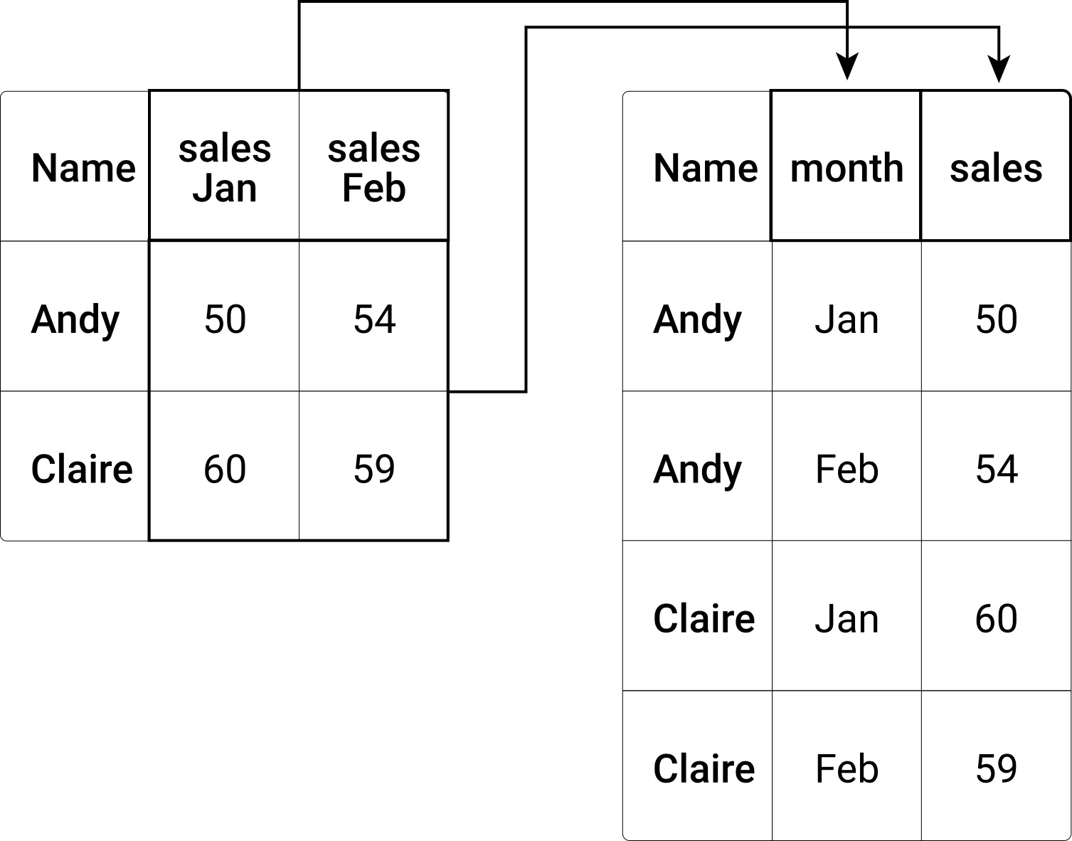
Figure 9.1: Reshaping of a data frame from wide to long format.

To illustrate how pivoting from wide to long works in practice, consider the following example dataset (extending on the example above).

wide_df <- data.frame(last_name = c("Wayne", "Trump", "Marx"),
                       first_name = c("John", "Melania", "Karl"),
                       gender = c("male", "female", "male"),
                       income.2018 = c("150000", "250000", "10000"),
                      income.2017 = c( "140000", "230000", "15000"),
                      stringsAsFactors = FALSE)
wide_df

##   last_name first_name gender income.2018 income.2017
## 1     Wayne       John   male      150000      140000
## 2     Trump    Melania female      250000      230000
## 3      Marx       Karl   male       10000       15000

The last two columns contain information on the same variable (income), but for different years. We thus want to pivot these two columns into a new year and income column, ensuring that columns correspond to variables and rows correspond to observations. For this, we call the pivot_longer()-function as follows:

long_df <- pivot_longer(wide_df, c(income.2018, income.2017), names_to = "year", values_to = "income")
long_df

## # A tibble: 6 × 5
##   last_name first_name gender year        income
##   <chr>     <chr>      <chr>  <chr>       <chr> 
## 1 Wayne     John       male   income.2018 150000
## 2 Wayne     John       male   income.2017 140000
## 3 Trump     Melania    female income.2018 250000
## 4 Trump     Melania    female income.2017 230000
## 5 Marx      Karl       male   income.2018 10000 
## 6 Marx      Karl       male   income.2017 15000

We can further clean the year column to only contain the respective numeric values.

long_df$year <- str_replace(long_df$year, "income.", "")
long_df

## # A tibble: 6 × 5
##   last_name first_name gender year  income
##   <chr>     <chr>      <chr>  <chr> <chr> 
## 1 Wayne     John       male   2018  150000
## 2 Wayne     John       male   2017  140000
## 3 Trump     Melania    female 2018  250000
## 4 Trump     Melania    female 2017  230000
## 5 Marx      Karl       male   2018  10000 
## 6 Marx      Karl       male   2017  15000

9.2.3 Pivoting from ‘long to wide’ (“spreading”)

As we want to adhere to the ‘tidy’ paradigm of keeping our data in long format, transforming ‘long to wide’ is less common. However, it might be necessary if the dataset at hand is particularly messy. The following example illustrates such a situation.

weird_df <- data.frame(last_name = c("Wayne", "Trump", "Marx",
                                     "Wayne", "Trump", "Marx",
                                     "Wayne", "Trump", "Marx"),
                       first_name = c("John", "Melania", "Karl",
                                      "John", "Melania", "Karl",
                                      "John", "Melania", "Karl"),
                       gender = c("male", "female", "male",
                                  "male", "female", "male",
                                  "male", "female", "male"),
                       value = c("150000", "250000", "10000",
                                 "2000000", "5000000", "NA",
                                 "50", "25", "NA"),
                       variable = c("income", "income", "income",
                                    "assets", "assets", "assets",
                                    "age", "age", "age"),
                       stringsAsFactors = FALSE)
weird_df

##   last_name first_name gender   value variable
## 1     Wayne       John   male  150000   income
## 2     Trump    Melania female  250000   income
## 3      Marx       Karl   male   10000   income
## 4     Wayne       John   male 2000000   assets
## 5     Trump    Melania female 5000000   assets
## 6      Marx       Karl   male      NA   assets
## 7     Wayne       John   male      50      age
## 8     Trump    Melania female      25      age
## 9      Marx       Karl   male      NA      age

While the data is somehow in a long format, the rule that each column should correspond to a variable (and vice versa) is ignored. Data on income, assets, and the age of the individuals in the dataset, are all put in the same column. We can call the function pivot_wider() with the two parameters names and value to correct this.

tidy_df <- pivot_wider(weird_df, names_from = "variable", values_from = "value")
tidy_df

## # A tibble: 3 × 6
##   last_name first_name gender income assets  age  
##   <chr>     <chr>      <chr>  <chr>  <chr>   <chr>
## 1 Wayne     John       male   150000 2000000 50   
## 2 Trump     Melania    female 250000 5000000 25   
## 3 Marx      Karl       male   10000  NA      NA

9.3 Stacking/row-binding datasets

In practice, you will encounter situations in which the raw data is partitioned according to one of the variables into separate data files. Typically, in the economics research context, this is done by date (sales records of a firm stored in one CSV file per month) or by geographic entities (e.g., one file with GDP per capita figures per country).

Unless the combined dataset of all separate files would be very large in memory, you likely would prefer one file to run analytics scripts on. Therefore, data preparation often also involves the stacking/binding of sub-sets into a larger combined dataset. As each of the separate files might slightly differ in terms of variable names, variable availability, and tidiness. It is important to first standardize/clean all of the separate datasets after importing them (following the examples above).

Once all of the subsets are imported an cleaned, there is typically still one remaining inconsistency: some variables might be available in some subsets (e.g., for some years, some regions) but not for others. In addition, the column/variable-order might vary between subsets.

Figure @refRow-binding/stacking three subsets into one combined dataset. illustrates the concept of stacking datasets (binding the rows of separate data frames) with some inconsistencies regarding the availability and order of columns.

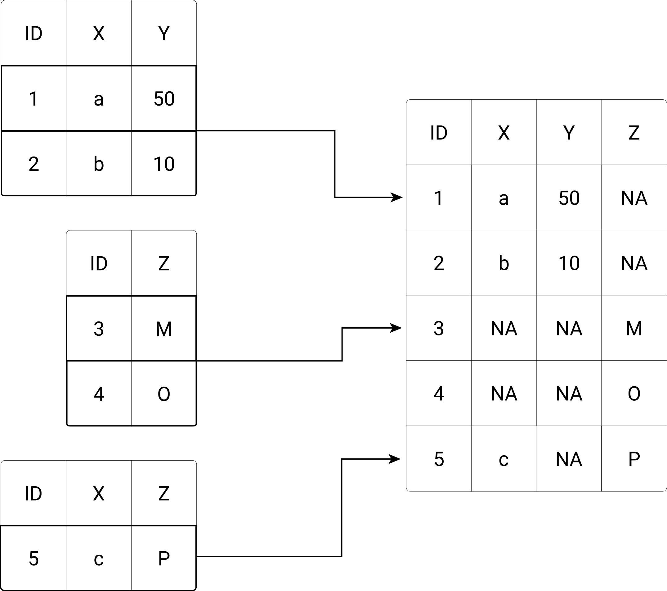
Figure 9.2: Row-binding/stacking three subsets into one combined dataset.

The dplyr-package provides an easy-to-use framework to implement such a stacking of data frames in R. In the following code illustration, we build on the same exemplary data as shown in the conceptual illustration above. First, we initiate the thee subsets, and then bind their rows to generate the combined dataset via bind_rows()

# initialize sample data
subset1 <- data.frame(ID=c(1,2),
                      X=c("a", "b"),
                      Y=c(50,10))

subset2 <- data.frame(ID=c(3,4),
                      Z=c("M", "O"))

subset3 <- data.frame(ID= c(5),
                      X=c("c"),
                      Z="P")

Note that, apart from the inconsistencies regarding the column availability and column order, the three subsets are consistent with each other in terms of basic data structure and data types (if that were not the case, binding their rows might be problematic).

str(subset1)

## 'data.frame':    2 obs. of  3 variables:
##  $ ID: num  1 2
##  $ X : chr  "a" "b"
##  $ Y : num  50 10

str(subset2)

## 'data.frame':    2 obs. of  2 variables:
##  $ ID: num  3 4
##  $ Z : chr  "M" "O"

str(subset3)

## 'data.frame':    1 obs. of  3 variables:
##  $ ID: num 5
##  $ X : chr "c"
##  $ Z : chr "P"

To stack the three subsets together, we call bind_rows() as follows (dplyr needs to be installed and loaded for this).

# install if needed
# install.packages("dplyr")

# load packages
library(dplyr)

# stack data frames
combined_df <- bind_rows(subset1, subset2, subset3)

# inspect the result
combined_df

##   ID    X  Y    Z
## 1  1    a 50 <NA>
## 2  2    b 10 <NA>
## 3  3 <NA> NA    M
## 4  4 <NA> NA    O
## 5  5    c NA    P

Note how bind_rows() automatically matches the column names (orders the columns before stacking), and fills missing values with NAs (not available).

9.4 Tutorial: Hotel Bookings Time Series

This tutorial guides you step-by-step through the cleaning script (with a few adaptions) of tidytuesday’s Hotel Bookings repo, dealing with the preparation and analysis of two datasets with hotel demand data. Along the way, you also get in touch with the janitor package. For details about the two datasets, see the paper by Nuno Antonio, de Almeida, and Nunes (2019), and for the original research contribution related to these datasets see the paper by N. Antonio, de Almeida, and Nunes (2017).

9.4.1 Background and aim

Nuno Antonio, de Almeida, and Nunes (2019) summarizes the content of the datasets as follows: “One of the hotels (H1) is a resort hotel, and the other is a city hotel (H2). Both datasets share the same structure, with 31 variables describing the 40,060 observations of H1 and 79,330 observations of H2. Each observation represents a hotel booking. Both datasets comprehend bookings due to arrive between the 1st of July 2015 and the 31st of August 2017, including bookings that effectively arrived and bookings that were canceled. Since this is real data, all data elements pertaining to hotel or customer identification were deleted. Due to the scarcity of real business data for scientific and educational purposes, these datasets can have an important role for research and education in revenue management, machine learning, or data mining, as well as in other fields.”

The aim of the tutorial is to get the data in the form needed for the following plot.

The first few rows and columns of the final dataset should combine the two source datasets and look as follows:

head(hotel_df)

## # A tibble: 6 × 32
##   hotel   is_ca…¹ lead_…² arriv…³ arriv…⁴ arriv…⁵ arriv…⁶ stays…⁷
##   <chr>     <dbl>   <dbl>   <dbl> <chr>     <dbl>   <dbl>   <dbl>
## 1 Resort…       0     342    2015 July         27       1       0
## 2 Resort…       0     737    2015 July         27       1       0
## 3 Resort…       0       7    2015 July         27       1       0
## 4 Resort…       0      13    2015 July         27       1       0
## 5 Resort…       0      14    2015 July         27       1       0
## 6 Resort…       0      14    2015 July         27       1       0
## # … with 24 more variables: stays_in_week_nights <dbl>,
## #   adults <dbl>, children <dbl>, babies <dbl>, meal <chr>,
## #   country <chr>, market_segment <chr>,
## #   distribution_channel <chr>, is_repeated_guest <dbl>,
## #   previous_cancellations <dbl>,
## #   previous_bookings_not_canceled <dbl>,
## #   reserved_room_type <chr>, assigned_room_type <chr>, …

9.4.2 Set up and import

All the tools we need for this tutorial are provided in tidyverse and janitor, and the data is directly available from the tidytuesday GitHub repository. The original data is provided in CSV format.

# SET UP --------------

# load packages
library(tidyverse)
library(janitor) # install.packages("janitor") (if not yet installed)

# fix variables
url_h1 <- "https://raw.githubusercontent.com/rfordatascience/tidytuesday/master/data/2020/2020-02-11/H1.csv"
url_h2 <- "https://raw.githubusercontent.com/rfordatascience/tidytuesday/master/data/2020/2020-02-11/H2.csv"

## DATA IMPORT -----------------

h1 <- read_csv(url_h1)
h2 <- read_csv(url_h2)

In the next step, we clean the column names and add columns to clarify which of the two hotels the corresponding observations belong to (see dataset description above). Finally, we stack the observations (rows) together in one tibble/data.frame.

## CLEAN DATA -------------------------

# use the janitor-package clean_names function. see ?clean_names for details
h1 <- clean_names(h1)
h2 <- clean_names(h2)

# add a column to clarify the origin of observation
h1 <- mutate(h1, hotel="Resort Hotel")
h2 <- mutate(h2, hotel="City Hotel")

# stack observations
hotel_df <- bind_rows(h1,h2)

# inspect the first observations
head(hotel_df)

## # A tibble: 6 × 32
##   is_ca…¹ lead_…² arriv…³ arriv…⁴ arriv…⁵ arriv…⁶ stays…⁷ stays…⁸
##     <dbl>   <dbl>   <dbl> <chr>     <dbl>   <dbl>   <dbl>   <dbl>
## 1       0     342    2015 July         27       1       0       0
## 2       0     737    2015 July         27       1       0       0
## 3       0       7    2015 July         27       1       0       1
## 4       0      13    2015 July         27       1       0       1
## 5       0      14    2015 July         27       1       0       2
## 6       0      14    2015 July         27       1       0       2
## # … with 24 more variables: adults <dbl>, children <dbl>,
## #   babies <dbl>, meal <chr>, country <chr>,
## #   market_segment <chr>, distribution_channel <chr>,
## #   is_repeated_guest <dbl>, previous_cancellations <dbl>,
## #   previous_bookings_not_canceled <dbl>,
## #   reserved_room_type <chr>, assigned_room_type <chr>,
## #   booking_changes <dbl>, deposit_type <chr>, agent <chr>, …

The option stringsAsFactors = FALSE ensures that all of the columns in this data frame are of type character.↩︎
If we perform the same operation on this variable before coercing it to a factor, this problem does not occur.↩︎
Depending on the dataset, however, an argument can be made that storing the data in wide format might be more efficient (using up less memory) than long format.↩︎