Introduction
“Are tomorrow’s bigger computers going to solve the problem? For some people, yes – their data will stay the same size and computers will get big enough to hold it comfortably. For other people it will only get worse – more powerful computers mean extraordinarily larger datasets. If you are likely to be in this latter group, you might want to get used to working with databases now.” (Burns 2011, 16)
At the center of Figure 3.1 you see an illustration of the key components of a standard local computing environment to process digital data. In this book, these components typically serve the purpose of computing a statistic, given a large dataset as input. In this part of the book, you will get familiar with how each of these components plays a role in the context of Big Data Analytics and how you can recognize and resolve potential problems caused by large datasets/large working loads for either of these components. The three most relevant of these components are:
Mass storage. This is the type of computer memory we use to store data over the long term. The mass storage device in our local computing environment (e.g., our PC/laptop) is generally referred to as the hard drive or hard disk.
RAM. In order to work with data (e.g., in R), it first has to be loaded into the memory of our computer – more specifically, into the random access memory (RAM). Typically, data is only loaded in the RAM for as long as we are working with it.
CPU. The component actually processing data is the Central Processing Unit (CPU). When using R to process data, R commands are translated into complex combinations of a small sets of basic operations, which the CPU then executes.
For the rest of this book, consider the main difference between common ‘data analytics’ and ‘Big Data Analytics’ to be the following: in a Big Data Analytics context, the standard usage of one or several of the standard hardware components in your local computer fails to work or works very inefficiently because the amount of data overwhelms its normal capacity.
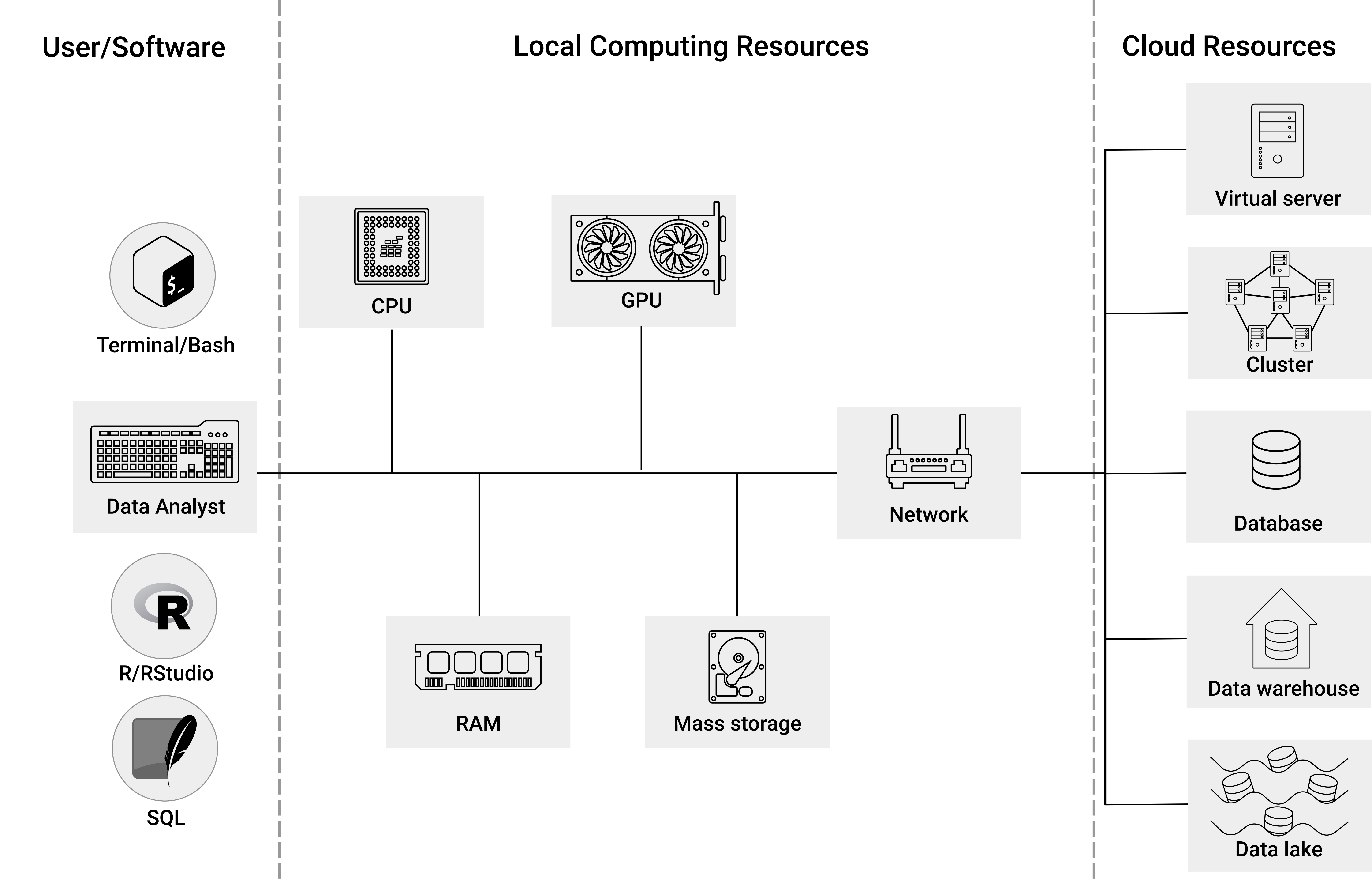
Figure 3.1: Software, local computing resources, and cloud resources.
However, before we discuss these hardware issues in Chapter 5, Chapter 4 focuses on the software we will work with to make use of these hardware components in the most efficient way. This perspective is symbolized in the left part of Figure 3.1. There will be three main software components with which we work in what follows. The first is the terminal (i.e., bash): instead of using graphical user interfaces to interact with our local computing environment, we will rather use the terminal9 to install software, download files, inspect files, and inspect hardware performance. For those of you not yet used to working with the terminal, do not worry! There are no prerequisites in knowledge about working with the terminal, and most of the use cases in this book are very simple and well explained. At this point, just note that there will be two types of code chunks (code examples) shown in what follows: either they show code that should be run in the terminal (in RStudio, such code should thus be entered in the tab/window called Terminal), or R code (in RStudio, this code should be entered in the Tab/window called Console).
R (R Core Team 2021) will be the main language used throughout this book. It will be the primary language to gather, import, clean, visualize, and analyze data. However, as you will already see in some of the examples in this part of the book, we will often not necessarily use base R, but rather use R as a high-level interface to more specialized software and services. On the one hand this means we will install and use several specialized R packages designed to manipulate large datasets that are in fact written in other (faster) languages, such as C. On the other hand, it will mean that we use R commands to communicate with other lower-level software systems that are particularly designed to handle large amounts of data (such as data warehouses, or software to run analytics scripts on cluster computers). The point is that even if the final computation is not actually done in R, all you need to know to get the particular job done are the corresponding R commands to trigger this final computation.
There is one more indispensable software tool on which we will build throughout the book, Structured Query Language (SQL), or to be precise, different variants of SQL in different contexts. The main reason for this is twofold: First, even if you primarily interact with some of the lower-level Big Data software tools from within R, it is often more comfortable (or, in some cases, even necessary) to send some of the instructions in the form of SQL commands (wrapped in an R function); second, while many of you might have only heard of SQL in the context of traditional relational database systems, SQL variants are nowadays actually used to interact with a variety of the most important Big Data systems, ranging from Apache Spark (a unified analytics platform for large-scale data processing) to Apache Druid (a column-based distributed data store) and AWS Athena (a cloud-based, serverless query service for simple storage/data lakes). Hence, if you work in data analytics/data science and want to seriously engage with Big Data, knowing your way around SQL is a very important asset.
Finally, Chapters 6 and 7 consider the situation where all of the tweaks to use the local computing resources most efficiently are still not enough to get the job done (one or several components are still overwhelmed and/or it simply takes too much time to run the analysis). From the hardware perspective, there are two basic strategies to cope with such a situation:
- Scale out (‘horizontal scaling’): Distribute the workload over several computers (or separate components of a system).
- Scale up (‘vertical scaling’): Extend the physical capacity of the affected component by building a system with a large amount of RAM shared between applications. This sounds like a trivial solution (‘if RAM is too small, buy more RAM…’), but in practice it can be very expensive.
Nowadays, either of these approaches is typically taken with the help of cloud resources (illustrated in the right part of Figure 3.1). How this is basically done is introduced in Chapter 7. Regarding vertical scaling, you will see that the transition from a local computing environment to the cloud (involving some or all of the core computing components) is rather straightforward to learn. However, horizontal scaling for really massive datasets involves some new hardware and software concepts related to what are generally called distributed systems. To this end, we first introduce the most relevant concepts related to distributed systems in Chapter 6.
References
To be consistent with the cloud computing services (particularly EC2) introduced later on, the sections involving terminal commands assume you work with Ubuntu Linux. However, the corrsponding code chunks are essentially identical for users working on a Mac/OSX-machine. In case you are working on a Windows machine, starting with Windows 10, you will have essentially the same tool available called the Windows Terminal. In older Windows versions the Linux terminal equivalent is called PowerShell or command prompt, which use a slightly different syntax, but provide similar functionality. See https://www.geeksforgeeks.org/linux-vs-windows-commands/ for an overview of how to get started with the Windows command prompt, including a detailed listing of commands next to their corresponding Linux command equivalents.↩︎